How we already said, we are going to comment in this post how to represent regressions with the command qplot.
Using the iris dataset, we are going to analyze several examples using various commands. To perform regressions it is mandatory to add the attribute geom=”smooth”. Although we can add more attributes.
Let's start by applying exclusively method = ”lm”, with which we obtain a line. That is to say, we will represent a linear regression. If we want to add a polynomial regression we have to add the attribute formula.
A continuación veremos cómo correlaciona lineamente el atributo Petal. Length (longitud del pétalo) con Sepal. Length (longitud del sépalo).
Escrbimos:
qplot(x=Sepal.Length, y=Petal.Length, data=iris, geom=(“smooth”), method=”lm”)
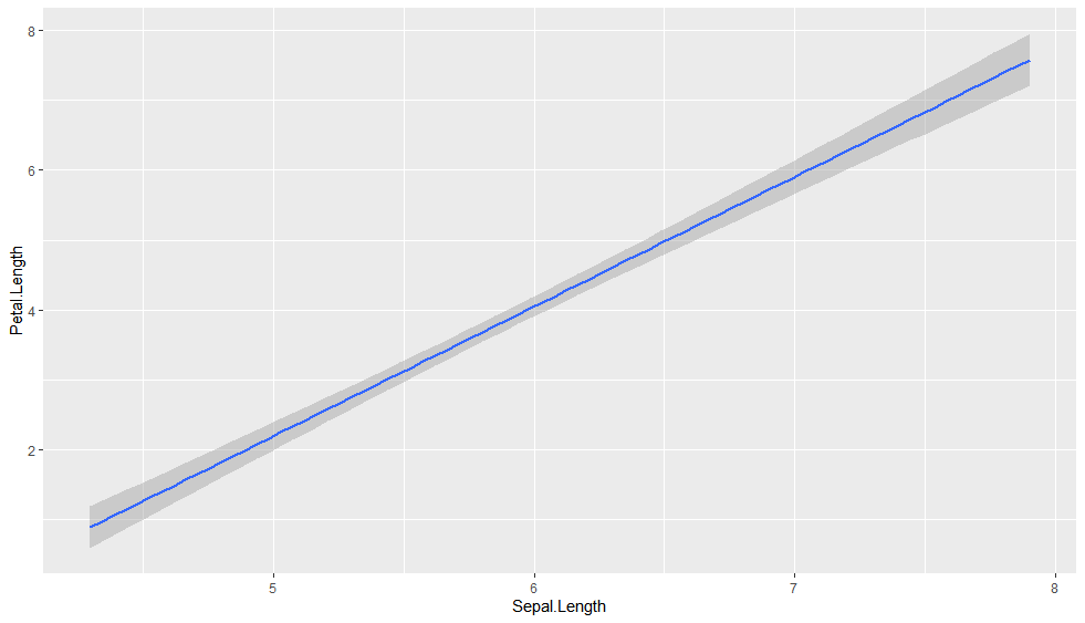
Vemos, que tomando las tres especies en conjunto, hay una clara correlación lineal, y de forma que la longitud del pétalo y sépalo suelen suelen ser muy similares.
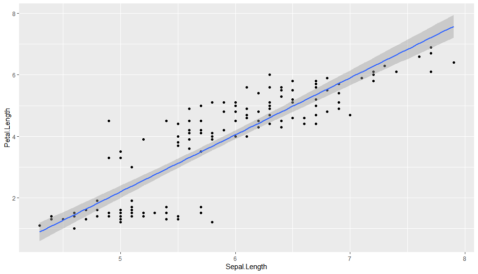
Ahora veámoslo pero representando también los valores cómo puntos. Escribimos:
qplot(x=Sepal.Length, y=Petal.Length, data=iris, geom=c(“point”, “smooth”), method=”lm”)
A continuación vamos a representar regresiones polinomiales. Para escribir fórmulas polinomiales en qplot lo tenemos que hacer de la siguiente forma:
1 degree: formula = y ~ x
2 degrees: formula = y~poly(x,2)
3 degrees: formula = y~poly(x,3)
n degrees: formula = y~poly(x,n)
Hagamos una representación de una regresión segundo grado, que correlacione Sepal. Length con Petal.Length:
qplot(x=Sepal.Length, y=Petal.Length, data=iris, geom=(“smooth”), method=”lm”, formula=y ~ poly(x,2))
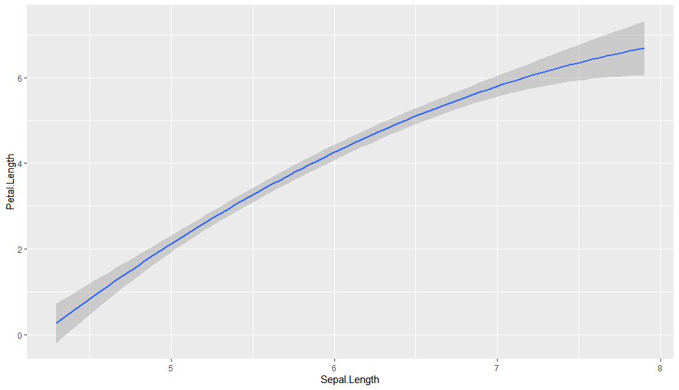
Now, una de tercer grado:
qplot(x=Sepal.Length, y=Petal.Length, data=iris, geom=(“smooth”), method=”lm”, formula=y ~ poly(x,3))

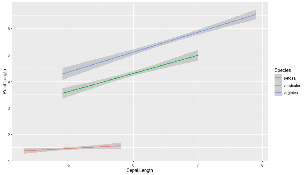
Para ver las rectas de regresión de las diferentes especies:
qplot(x=Sepal.Length, y=Petal.Length,data=iris,geom=”smooth”,method=”lm”, color=Species )
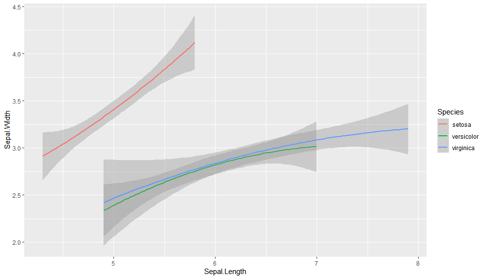
Now, lo mismo pero con una regresión polinomial de grado 2, y comparando la longitud del sépalo ( Sepal.Length) con su anchura ( Sepal.Width).
qplot(x=Sepal.Length, y=Sepal.Width, data=iris, geom=(“smooth”),method=”lm”, formula=y ~ poly(x,2), color=Species)
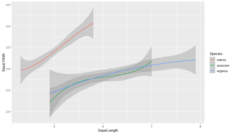
Lo mismo pero con una regresión de tercer grado:
qplot(x=Sepal.Length, y=Sepal.Width, data=iris, geom=(“smooth”),method=”lm”, formula=y ~ poly(x,3), color=Species)
Y hasta aquí esta entrada. En la próxima, seguiremos explorando las posibilidades del paquete ggplot2.